Model Free Adaptive Control Theory and Applications Reviews Google Reads

Commodity Menu

/ajax/scifeed/subscribe

Open Access Article

Information-Driven Model-Costless Adaptive Control of Z-Source Inverters

^one

Department of Electrical Applied science, Shahid Bahonar University of Kerman, Kerman 7616913439, Iran

ⁱⁱ

Section of Electrical and Software Engineering, University of Calgary, Calgary, AB T2N 1N4, Canada

³

Section of Electrical and Calculator Engineering, Sharif University of Technology, Tehran 1136511155, Iran

⁴

School of Engineering, Royal Melbourne Institute of Engineering, Melbourne 2476, Australia

⁵

Department of Mathematics, Physics and Electrical Applied science, Northumbria University, Newcastle NE7 7XA, UK

^{half dozen}

Department of Electrical Engineering, Academy of Tabriz, Tabriz 5166616471, Iran

^*

Authors to whom correspondence should be addressed.

Academic Editor: Carlos Silvestre

Received: 20 September 2021 / Revised: one November 2021 / Accepted: 3 November 2021 / Published: 9 Nov 2021

Abstract

The universal prototype shift towards green energy has accelerated the evolution of modern algorithms and technologies, among them converters such as Z-Source Inverters (ZSI) are playing an important role. ZSIs are unmarried-stage inverters which are capable of performing both buck and heave operations through an impedance network that enables the shoot-through state. Despite all advantages, these inverters are associated with the non-minimum phase feature imposing heavy restrictions on their airtight-loop response. Moreover, uncertainties such every bit parameter perturbation, unmodeled dynamics, and load disturbances may degrade their functioning or even lead to instability, especially when model-based controllers are applied. To tackle these bug, a data-driven model-free adaptive controller is proposed in this paper which guarantees stability and the desired performance of the inverter in the presence of uncertainties. It performs the control action in ii steps: First, a model of the arrangement is updated using the current input and output signals of the arrangement. Based on this updated model, the control activity is re-tuned to achieve the desired performance. The convergence and stability of the proposed control system are proved in the Lyapunov sense. Experiments corroborate the effectiveness and superiority of the presented method over model-based controllers including PI, state feedback, and optimal robust linear quadratic integral controllers in terms of various metrics.

one. Introduction

Penetration of renewable energy resource has changed the construction of power systems toward distributed generation. To have a smooth and reliable transition in this image shift, several technical and non-technical problems should be solved [1,2,3]. Inverters are 1 of the core components of future power grids with several applications in connecting batteries to grid, maximum ability point tracking of solar panels, and smart grids [four]. Among different types of inverters, the buck-boost inverter is highly demanded due to lower stress on its components during operation as well as voltage increment/decrease capabilities [5,6]. However, traditional ii-stage buck-heave inverters have the potential of short/open-circuit which abstention requires time/overlap delays to be added in their functioning. This indeed results in a higher cost, lower efficiency, more complexity, and a slight distortion in output waveforms [7].

To recoup for this drawback, Z-source inverters (ZSI) accept been proposed which can operate in either voltage or current source modes [8]. They use both buck and heave operations in one single-stage topology [9], using fewer switching devices [vii], which results in a simple design and a high efficiency [10]. The shoot-through state of the ZSI is triggered by charging/discharging of capacitors and inductors in an X-shaped impedance circuit [eleven]. ZSIs have attracted a lot of research activities during recent years due to their applications in electric vehicles [12], wind power [13], and battery energy storage systems [14].

Several control methodologies, such as PI controllers [xv], model predictive command (MPC) [16], fuzzy control [17], and sliding manner control [18], take been practical to ameliorate their performance. While the experimental implementation of the fuzzy controller is also complicated [19], a LMI-based design method was introduced in Amirhossein et al. [20] to ensure Lyapunov stability of the inverter in the presence of uncertainties also as keeping the desired level of disturbance rejection. The control and implementation of a bidirectional ZSI for a standalone hybrid system including PV, a diesel generator, and an energy storage organization is explored in [21]. The current ripple of ZSI is analyzed and controlled in Shuai et al. [22] using an adjustable DC-link voltage and switching frequency strategy. A fractional-lodge PID controller is adopted in [23] for a bidirectional quasi-ZSI used in electric traction system, which is optimized using an emmet colony optimization algorithm. Robust and fast control of a ZSI-based interior permanent magnet synchronous motor drive system is developed in Ghahderijani and Dehkordi [24] using the sliding mode command as the feedback controller empowered by a disturbance attenuation feed-forward compensator. Furthermore, a robust linear quadratic integral controller was recently introduced in Ahmadi et al. [11] for ZSIs subject field to uncertainties, using the bat algorithm based on instantaneous exploitation [25].

Despite these advances, the Not-Minimum Stage (NMP) feature of ZSIs in improver to natural uncertainties which happen in different operating conditions severely impact the performance of linear control approaches. Although the NMP behavior can exist modeled equally a time delay, i.e.,

$1-\tau s=e^{-\tau s}$

[26,27], information technology causes both undershoot and overshoot in the transient response, escalates the harmonic distortions, and may lead to instability. The model-based predictive strategies, such as MPC, have shown the capability of dealing with NMP systems. Nevertheless, they are non robust plenty against variation of parameters.

The majority of control strategies that have been exerted on power electronic devices in the literature are based on a mathematical model of the system [xi]. Generally, these models suffer from lack of unmodeled dynamics and precise cognition of uncertainties, such as variation of load in electric vehicles. It is well-known that components of renewable free energy systems, such as ZSI, are subject to persistent uncertainties [28]. This means that model-based controllers that are designed based on these models may upshot in a poor performance in practice [29]. In other words, it is not possible to ascertain the practicality of most of the theoretical model-based results of a closed-loop control system (e.g., stability and convergence) [xxx]. I solution is using robust controllers like non-fragile

$H_{\infty }$

multivariable PID controller [31], which requires complicated and bourgeois pattern procedure. Nevertheless, thanks to advancements in informatics and sensing technologies, a large amount of data has been generated and stored in many industrial processes, preserving all the useful state data of the process operations and equipment [32]. Therefore, the idea of compensating for incomplete mathematical models using process data has emerged. In fact, in cases where precise procedure models are not bachelor, data can exist used for controller pattern, prediction, diagnosis, and assessment of the industrial processes.

Inspired past this idea, the concept of data-driven command (DDC) has attracted much attention during recent years. It employs the Input and Output (I/O) measurements of the institute to prepare the appropriate control control [33]. Several data-driven methods take been developed so far including PID command, iterative feedback tuning, model-complimentary adaptive control (MFAC), iterative learning, and virtual reference feedback control [34]. Although design and stability analysis of DDC methods is generally complicated, they have shown strong performance in tackling uncertainties, nonlinearities, and even cyber attacks to industrial systems [35]. It means that they can exist advisable solutions for control of ZSIs. Based on this, MFAC is practical to ZSI in this paper when uncertainties, including parameters perturbation, unmodelled dynamics, and external disturbances exist. More often than not, MFAC is designed for effective control of discrete-time nonlinear systems [36,37], which is the case for ZSI. Several theoretical and experimental results for nonlinear multi-input-multi-output systems have been reported using MFAC, encounter, due east.thousand., in Roman et al. [38], Xu et al. [39], Liang et al. [xl]. This method is based on a dynamical linearization data model of the plant. A dynamic linearization method, incorporating the pseudo-partial derivative (PPD), places these data models at every dynamic performance point in the closed-loop system.

In this paper, ZSI is starting time faux in different operating modes and its country-space model is obtained using input and output signals. As the model is updated online while the command organization is running, this model includes uncertainties of the system as well. Then, a information-driven model-free adaptive controller is proposed for the organization to guarantee stability and provide the desired performance. Indeed, this controller updates the command command based on the system model that is updated using latest input and out signals. The convergence and stability of the proposed control system are mathematically proved in the Lyapunov sense. To have a improve evaluation, the performance of the proposed controller in managing nonlinearities, uncertainties, and the NMP beliefs is compared with other controllers including PI, state-feedback (SF), and optimal robust linear quadratic integral (LQI) controller [11]. Simulation results evidence that the proposed controller successfully damps the external disturbance, tackles uncertainties, and provides a better transient response compared to its peers.

The remaining parts of this paper are structured equally follows. Section ii illustrates the excursion analysis and land-space model of the ZSI. In Section 3, a discussion of the proposed method is provided and the closed-loop stability of the control system is proved. Section 4 presents simulation results to establish the efficiency of the proposed controller. Finally, Section 5 briefly concludes the paper.

2. Excursion Assay

ZSI is a blazon of cadet-boost ability inverter with an extraordinary topology which does non crave the well-known DC-DC converter bridge. Impedance Z-source networks efficiently facilitate the power conversion from the source to the load and are extensively applicable in numerous electric power conversion systems [41]. Effigy 1 shows the topology of a three-phase voltage-fed ZSI constructed by the DC power source

$V_{in}$

; a Z-source network including

${\mathrm{Fifty}}_1$

,

$L_2$

,

$C_1$

,

$C_2$

, and r; and a load which tin can be shown by

$R_o$

and

$L_o$

. The desired value might be accomplished by changing the shoot-through duty ratio. Considering different switching states, the ZSI of Effigy 1a can work in two modes: non-shoot-through and shoot-through modes. The country vector

$\mathrm{10}={[i_L,v_C,i_o]}^T$

can be used in deriving dynamical equations of these two modes, where

${\mathrm{five}}_c$

,

$i_L$

, and

$i_o$

show the capacitor voltage, inductor current, and output current, respectively. The parasitic resistance of inductors is represented by r.

2.1. Shoot-Through Fashion

In addition to the traditional six active and two zero states in the dynamical model, the ZSI incorporates a shoot-through zero state in order to increment voltage. The detailed operation of these states has been presented in Shen and Peng [42]. More often than not, when the agile states remain unchanged, just the naught states incorporate the shoot-through mode, and with a small modification in the zero states, an Ac output voltage of the inverter will still resemble a traditional inverter besides the traditional PWM modulation methods. To accept a better comprehension, in Figure 2 the overall method of boost PWM modulation is presented. The allocation of the shoot-through naught vectors for each phase eventually takes place with the total zero-vector time interval remaining unchanged. Therefore, interpolating shoot-through aught vectors enhances the DC-link voltage with no changes to the agile-vector time. Here, the switching frequency is

$f=1/T_{\mathrm{southward}}$

in which

$T_{\mathrm{south}}=T_{sh}+T_n$

. The shoot-through and non-shoot-through intervals are shown by

$T_{\mathrm{due\; south}h}$

and

$T_n$

, respectively, and the shoot-through duty cycle is

$d=T_{\mathrm{south}h}/(T_{sh}+T_n)$

. As depicted in Figure 1c, in this mode, a mixture of lower and upper switches shortens the output terminals of the inverter. Furthermore, the diode is here reversely biased, meaning that the circuit is disconnected from the power system and inductors are charged past the stored energy in capacitors. Taking reward of the shoot-through duty ratio and the free energy transfer, the boosting capability of the ZSI has emerged. Here, the voltages throughout the inductors and DC-link are

$v_L=v_c$

and

$v_{dc}=0$

. This mode is expressed in the following state-space model.

$$\dot{\mathrm{ten}}=\underset{A_{sh}}{\underbrace{\left[\begin{array}{ccc}-\frac{r}{L}& \frac{\mathrm{one}}{L}& 0\\ -\frac{1}{C}& 0& 0\\ 0& 0& -\frac{R_o}{{\mathrm{Fifty}}_o}\end{array}\right]}}\mathrm{x}$$

(1)

In the in a higher place equation, the effects of the input voltage power is omitted due to the diode changed bias beliefs.

2.2. Not-Shoot-Through Manner

In this style, the energy is conveyed through the inductors and input source to attain the load and capacitors as shown in Figure 1b. The post-obit mathematical model expresses the ZSI operation in this mode.

$$\dot{\mathrm{x}}=\underset{A_n}{\underbrace{\left[\begin{array}{ccc}-\frac{r}{\mathrm{Fifty}}& -\frac{1}{L}& 0\\ \frac{\mathrm{one}}{C}& 0& -\frac{1}{C}\\ 0& \frac{\mathrm{two}}{{\mathrm{Fifty}}_o}& -\frac{R_o}{{\mathrm{Fifty}}_o}\end{array}\right]}}\mathrm{ten}+\underset{B_{\mathrm{northward}}}{\underbrace{\left[\begin{array}{c}\frac{1}{L}\\ 0\\ -\frac{\mathrm{one}}{L_o}\end{array}\right]}}{V}_{in}$$

(ii)

Based on the circuit law, the voltages across inductors and the DC link are

$5_L={\mathrm{Five}}_{in}-{\mathrm{Five}}_C$

and

${\mathrm{Five}}_{dc}=V_C-V_L=2{\mathrm{Five}}_C-5_{i\mathrm{north}}$

, respectively. The duty bike in this mode is

$1-d$

. By using the State-Infinite Averaging (SSA) technique, i may accomplish

$$\dot{\mathrm{x}}=(A_n\times (\mathrm{i}-d)+A_{sh}\times d)\mathrm{x}+(B_n\times (1-d)+B_{\mathrm{due\; south}h}\times d)V_{in}$$

(3)

Consequently, the global state-space model is gained by substituting (ane) and (2) in (3) as follows:

$$\dot{\mathrm{x}}=\left[\begin{array}{ccc}-\frac{r}{\mathrm{Fifty}}& \frac{2d-1}{\mathrm{Fifty}}& 0\\ -\frac{2d-\mathrm{ane}}{C}& 0& -\frac{\mathrm{one}-d}{C}\\ 0& \frac{\mathrm{two}(1-d)}{C}& -\frac{R_o}{L_o}\end{array}\right]\mathrm{ten}+\left[\begin{array}{c}\frac{1-d}{L}\\ 0\\ -\frac{\mathrm{i}-d}{L_o}\end{array}\right]V_{i\mathrm{north}}$$

(4)

Because

$r=0$

, which is a known approximation in the literature [11], Equation (4) becomes

$$V_C=\frac{\mathrm{ane}-D}{1-2D}{V}_{i\mathrm{northward}}$$

(5)

in which D denotes the steady-land value of d. The average voltage across DC-link can exist written as

$$V_{dc}=(\mathrm{one}-D)\times (\mathrm{two}{V}_C-V_{in})+D\times 0=\frac{1-D}{1-\mathrm{two}D}{V}_{in}$$

(vi)

Therefore, the relationship between the DC-link voltage and

${\mathrm{Five}}_{in}$

becomes

$$v_{dc}=2V_C-V_{i\mathrm{northward}}=\frac{1}{\mathrm{one}-2D}{V}_{i\mathrm{northward}}=B{V}_{in}$$

(vii)

where

$B=\mathrm{i}/(1-2D)$

is the boosting factor. As indicated in (seven), the peak output voltage of the ZSI is illustrated as follows:

$$v_{ac}=M\frac{v_{dc}}{\mathrm{ii}}=\mathrm{Grand}B\frac{{\mathrm{Five}}_{i\mathrm{north}}}{2}$$

(eight)

in which M is the modulation index. This indicates that, despite traditional inverters, ZSI could work in the buck mode and reach the desired voltage by merely tuning an additional adjustable parameter similar B.

three. The Proposed Controller

In order to deal with complexities of nonlinear systems, the employ of the linearization techniques such every bit feedback linearization, Taylor's linearization, and piecewise linearization [33] is popular. These approaches may result in sophisticated models which are non appropriate for controller blueprint. For instance, the orthogonal function-based approximation method would result in a model with many parameters or of a very high order. A model, which is linearized for data-driven control applications, should have a elementary construction, moderate number of adaptable parameters, and convenient utilization of I/O data. Therefore, in this article, a new Compact Course Dynamic Linearization (CFDL) is employed in which the constraints play the office of inputs. In add-on, the CFDL method is essentially concerned about how changes in the current input betoken results in the variation of the output point in the next time instant, thus advisable for dynamical systems. A class of SISO nonlinear discrete-fourth dimension systems is considered every bit

$$y(h+\mathrm{ane})=f(y\left(h\right),\dots ,y(h-{\mathrm{northward}}_y),u\left(h\right),\dots ,u(h-n_u))$$

(nine)

where

$u\left(h\right)\in R$

and

$y\left(h\right)\in R$

are input and output of the system at time instant h, respectively;

$n_u$

and

$n_y$

are unknown positive integers; and

$f(·):R^{(n_u+n_y+\mathrm{two})}\to R$

is the unknown nonlinear function. Earlier expanding the CFDL model, some assumptions are required.

Assumption1.

The fractional derivative of $f(·)$ regarding the $(n_y+2)$th variable is continuous for all h with finite exceptions.

Supposition2.

Organisation (9) meets the generalized Lipschitz condition for all h with finite exceptions. This can exist expressed as

$$|y(h_1+1)-y(h_2+1)|\le b|u\left(h_1\right)-u\left(h_{\mathrm{ii}}\right)|$$

(10)

where $u\left(h_{\mathrm{one}}\right)\ne u\left(h_2\right)$ if $h_1\ne h_{\mathrm{ii}}$, $h_1,h_2>=0$, and b is a positive constant. We besides have $y(h_i+\mathrm{one})=f(y\left(h_i\right),\dots ,y(h_i-n_y),u\left(h_i\right),\dots ,u(h_i-n_u))$ for $i=\mathrm{i},2$.

These assumptions are adequately practical. Assumption 1 is very reasonable in many control systems, and Supposition 2 from an free energy perspective means that the rate of modify of free energy in the system is limited by a factor of the input energy to the system. These assumptions are satisfied for many practical systems such as pressure or temperature control systems, power systems, and fluid level control systems. For the sake of abbreviation, the argument "for all h with finite exceptions" is omitted in the subsequent results.

Theorem1.

Suppose that system (9) satisfies the Assumptions 1 and 2, and $|\Delta u(h\left)\right|\ne 0\forall h$. There exists a time-varying parameter ${\vartheta }_c\left(h\right)\in R$ which transforms the above system to the following CFDL:

$$\Delta y(h+\mathrm{i})={\vartheta }_c\left(h\right)\Delta u\left(h\right)$$

(xi)

where ${\vartheta }_c\left(h\right)<\delta$ is bounded at whatever time h. The proof of this theorem was illustrated in item in [37].

Remark1.

Theorem one requires that $|\Delta u(h\left)\right|\ne 0$ for all h. In reality, if $|\Delta u(h\left)\right|=0$ occurs at a specific fourth dimension, linearization can exist practical after a fourth dimension shift.

All the nonlinear properties of the organization are illustrated in

${\vartheta }_c\left(h\right)$

. Obtaining the mathematical model of

${\vartheta }_c\left(h\right)$

directly can exist very complex. Withal, its numerical behavior is obtained through nonlinear parameter recognition algorithms. For a SISO system such as

$y(h+1)=f\left(u\right(h\left)\right)$

, the pseudo-partial derivative (PPD) represents the value of the derivative of the role f at a given point of f at a given bespeak in the range of h to

$h+1$

. When PPD is upper bounded, no sharp modify is possible in the nonlinear office.

3.1. Algorithm of the Controller

The design algorithm of the MFAC is discussed in this subsection. A dynamic linear model corresponding to the nonlinear system is considered showtime. Then, the online input and output data is used to evaluate PDD, and the controller is designed such that a cost function is minimized. The price part is

$$J\left(u\left(h\right)\right)={|R(h+\mathrm{one})-y(h+\mathrm{i})|}^2+\lambda {|u\left(h\right)-u(h-1)|}^2$$

(12)

In this price function,

$\lambda >0$

represents the penalisation factor that prevents the control signal from rapid changes, and R shows the reference signal. Substituting

$y(h+1)=y\left(h\right)+{\vartheta }_c\left(h\right)\Delta u\left(h\right)$

in this toll function and using the Lagrange equation, the optimal control signal can be obtained, using derivation relative to u, equally follows:

$$u\left(h\right)=u(h-1)+\frac{\rho {\vartheta }_c\left(h\right)}{\lambda +|{\vartheta }_c{\left(h\right)|}^2}(R(h+\mathrm{one})-y\left(h\right))$$

(13)

The parameter

$\rho \in (0,1]$

can make the algorithm more than comprehensive, which is used to prove the stability in Hou and Jin [37].

Remark2.

As mentioned in a higher place, λ is a punishment factor in the cost function that prevents rapid changes in the control signal. As an essential tunable parameter in MFAC, the right setting of λ reduces the tracking fault.

3.2. Estimation Algorithm of PPD

Theorem ane shows that the the dynamic linearization model tin exist applied for nonlinear system (nine) whenever Assumptions i and 2 are satisfied. In add-on, Equation (16) shows that the optimal control signal can be accurately obtained if the PPD value is known. However, finding the exact PPD value from the model is difficult. An optimal PPD minimizes the cost function

$$J\left({\vartheta }_c\left(h\right)\right)=\mid y\left(h\right)-y(h-\mathrm{i})-{\vartheta }_c\left(h\right)\Delta u(h-\mathrm{one}){\mid }^2+\mu \mid {\vartheta }_c\left(h\right)-{\widehat{\vartheta }}_c(h-1){\mid }^2$$

(14)

in which

$\mu >0$

is a weight coefficient. From the optimal control theory, the value of

${\widehat{\vartheta }}_c$

is obtained every bit

$${\widehat{\vartheta }}_c\left(h\right)={\widehat{\vartheta }}_c(h-\mathrm{ane})+\frac{\theta \Delta u(h-1)}{\mu +\Delta u{(h-\mathrm{one})}^2}(\Delta y\left(h\right)-{\widehat{\vartheta }}_c(h-1)\Delta u(h-1))$$

(xv)

in which

$\theta \in (0,\mathrm{one})$

denotes a step-size constant. Finally, the full general form of CFDL-MFAC is given by

$${\widehat{\vartheta }}_c\left(h\right)={\widehat{\vartheta }}_c(h-1)+\frac{\theta \Delta u(h-1)}{\mu +\Delta u{(h-1)}^2}(\Delta y\left(h\right)-{\widehat{\vartheta }}_c(h-\mathrm{one})\Delta u(h-1))$$

(16)

$$u\left(h\right)=u(h-1)+\frac{\rho {\widehat{\vartheta }}_c\left(h\right)}{\lambda +|{\widehat{\vartheta }}_c{\left(h\right)|}^2}(R(h+1)-y\left(h\right))$$

(17)

There is a reset mechanism to forbid the interpretation algorithm from falling asleep and is implemented using

${\widehat{\vartheta }}_c\left(h\right)={\widehat{\vartheta }}_c\left(1\right)$

, if

${\widehat{\vartheta }}_c\left(h\right)\le \mathrm{east}$

or

$\mathrm{south}ign\left({\widehat{\vartheta }}_c\left(h\right)\right)\ne si\mathrm{1000}\mathrm{north}\left({\widehat{\vartheta }}_c\left(\mathrm{ane}\right)\right)$

. Figure 3c shows the cake diagram of the proposed controller.

3.iii. Stability Analysis

Theorem2.

Suppose the nonlinear organisation (9) is controlled using the controller (17) and the model update machinery (sixteen), under Assumptions 1 and 2 . In regulation problem, that is, $R(h+1)=R\left(h\right)$, there exists a constant ${\lambda }_{\mathrm{one\; thousand}i\mathrm{due\; north}}$ such that the regulation functioning is satisfactory for all $\lambda >{\lambda }_{mi\mathrm{north}}$. It means that $li{\mathrm{chiliad}}_{h\to \infty }|R(h+1)-y\left(h\right)|=0$.

Proof.

We prove the theorem in two steps: In step 1, the boundedness of the pseudo-Jacobian matrix estimation

${\widehat{\vartheta }}_c\left(h\right)$

is proved. So, the convergence of the tracking error and the BIBO stability of the DDC system are shown.

Step 1: This step is already proved in Hou and Jin [37].

Step ii: In this pace, we bear witness that the output tracking error

$\epsilon \left(h\right)=R\left(h\right)-y\left(h\right)$

is bounded. Because the Lyapunov role

$V\left(h\right)={\epsilon }^T\left(h\right)\epsilon \left(h\right)$

, 1 can achieve

$$\Delta V(h+\mathrm{i})={\epsilon }^T(h+\mathrm{one})\epsilon (h+\mathrm{i})-{\epsilon }^T\left(h\right)\epsilon \left(h\right)$$

(18)

where

$\epsilon (h+1)=R(h+1)-y(h+1)$

. For the regulation trouble, i.east., when

$R(h+1)=R\left(h\right)$

, (13) is expressed as

$$\epsilon (h+1)=R(h+\mathrm{ane})-y\left(h\right)-{\vartheta }_c\left(h\right)\rho \frac{{\widehat{\vartheta }}_c^T\left(h\right)(R(h+1)-y\left(h\right))}{\lambda +|{\widehat{\vartheta }}_c{\left(h\right)|}^2}$$

(xix)

in which,

$\epsilon (h+\mathrm{one})=H\left(h\right)\epsilon \left(h\right)$

and

$H\left(h\right)=I_m-{\vartheta }_c\left(h\right)\rho \frac{{\widehat{\vartheta }}_c^T\left(h\right)}{\lambda +|{\widehat{\vartheta }}_c{|}^2}$

. Therefore,

$$\begin{array}{cc}\hfill \Delta V(h+\mathrm{one})=& {\epsilon }^T\left(h\right)H^T\left(h\right)H\left(h\right)\epsilon \left(h\right)-{\epsilon }^T\left(h\right)\epsilon \left(h\right)\hfill \\ \hfill =& {\epsilon }^T\left(h\right)[H^T\left(h\right)H\left(h\right)-I_m]\epsilon \left(h\right)\hfill \end{array}$$

(20)

To prove the stability, it is sufficient to prove that the

$|H(h)|<\mathrm{i}$

. We have

$$|I_{\mathrm{yard}}-{\vartheta }_c\left(h\right)\rho \frac{{\widehat{\vartheta }}_c^T\left(h\right)}{\lambda +|{\widehat{\vartheta }}_c{\left(h\right)|}^2}|<1$$

(21)

which leads to

$$|{\vartheta }_c\left(h\right)\rho \frac{{\widehat{\vartheta }}_c^T\left(h\right)}{\lambda +|{\widehat{\vartheta }}_c{|}^2}|\le |\rho ||{\vartheta }_c||\frac{\mathrm{ane}}{2\sqrt{{\lambda }_{\mathrm{thou}i\mathrm{due\; north}}}}|$$

(22)

Considering the boundedness of

$\rho$

and

$\delta$

, there exist a positive

${\lambda }_{\mathrm{yard}in}$

such that

$$|{\vartheta }_c\left(h\right)\rho \frac{{\widehat{\vartheta }}_c^T\left(h\right)}{\lambda +|{\widehat{\vartheta }}_c{|}^2}|\le |\frac{\rho \delta }{2\sqrt{{\lambda }_{mi\mathrm{northward}}}}|<\mathrm{i}$$

(23)

which completes the proof. □

iv. Simulation Result

Suppose a load is supplied by an input voltage of xx 5 through a ZSI that operates at v kHz and incorporates a simple-boost PWM. The load is a three-phase l Hz, 55 V (line), 5 A, and Y-connected with a 0.viii lagging power gene. System parameters are shown in Tabular array one and are based on those in Hou and Jin [37]. Parametric uncertainties are considered in the load and the shoot-through duty cycle as

$R_o\in [10,60]$

and

$D\in [0.3,1]$

, respectively. The functioning and robustness of the proposed controller are compared with a PI controller, a SF controller, and an optimal robust LQI controller. Figure 3a shows the PI controller within dual loop schemes. A simple integral activeness is used in the outer loop while the parameters of the inner PI controller are [xi]

$$PI=k_i/\mathrm{south},k_i=0.0564$$

(24)

The SF controller is designed as [11]

$$K=[-0.00070.0031-0.071-0.0211]$$

(25)

$$d\left(t\right)=-0.0007i_{\mathrm{Fifty}}+0.00315_C-0.071i_o-0.021x_{ext}$$

(26)

The LQI controller can as well be designed as [eleven]

$$\mathrm{One\; thousand}=[0.62410.0153-0.1468-22.3607]$$

(27)

$$d\left(t\right)=0.6241i_L+0.0153v_C-0.1468i_o-22.3607{\mathrm{ten}}_{e\mathrm{10}t}$$

(28)

The initial conditions of the proposed controller are

$u\left(1\right)=u\left(2\right)=u\left(\mathrm{three}\right)=0$

,

$-y\left(1\right)=y\left(2\right)=y\left(3\right)=\mathrm{one}$

, and

${\vartheta }_c\left(1\right)=20000$

, and the step factors are

$\rho =\mathrm{0.six}$

,

$\theta =\mathrm{0.i}$

,

$\lambda =0.5$

, and

$\mu =0.2$

.

Performance of these controllers are compared with our proposed DDC ane in the nominal condition, in the presence of perturbations, and also in the example of load fluctuations. Figure iv shows the variations of the capacitor voltage

$v_C$

and the output current

$i_o$

acquired past a 4A load disturbance. The nominal operating condition is considered to happen for

$D=0.4374$

and

$R_o=27$

. This figure shows that all of the controllers respond in a stable regulatory way with servomechanism and no constant error. However, in the undershoot beliefs, the difference betwixt SF, PI, and LQI controllers with the proposed method is notable since our DDC controller does not have whatever undershoot due to its prediction capability. Furthermore, in the disturbance rejection comparison, the proposed method is too powerful and damps the external disturbance in a short time. As is observed, the capacitor has reached the constant voltage of 89.8 Five, slightly different from the expected 89.8146. The output electric current obtained is 4.236, again with only a slight divergence from the expected 4.2362. Also, for the applied operation of the ZSI, the smoothness of the controllers is validated by TV metric. To better compare operation of these controllers, Table 2 summarizes the performance indices for these controllers.

To compare the robustness of controllers against variations in constitute parameters, the previous parameter setting is incorporated in stimulation with disturbances. In Figure five,

$v_C$

and

$i_o$

are compared when the arrangement parameters are perturbed to

$D=0.45$

and

$R_o=\mathrm{sixty}$

, comparing to the nominal condition

$D=0.4347$

and

$R_o=27$

. A 4A load fluctuation is practical to the organization and functioning of unlike controllers are compared. Figure 5 shows stable performance of all controller, except PI, in this case. The proposed MFAC controller maintains the closed-loop response and provides a high robustness against parameter variations. Finally, the last simulation is performed in the perturbed condition (

$D=\mathrm{0.four}$

,

$R_o=60$

) to investigate reliability. It could exist seen in Effigy half dozen that SF and PI controllers no longer produce a satisfactory transient response and lead to depression-frequency large or high-frequency minor oscillations when rejecting disturbances. This means that a small parameter perturbation in D considerably impacts performance of these two controllers. The figure also shows that the proposed DDC is potent plenty to reject this disturbance. This is mainly because of the model update mechanism and adaptive behavior of the controller. To better compare performance of these controllers, Table iii and Table 4 summarize the performance indices for different perturbed conditions.

v. Conclusions

ZSIs have several potential applications in renewable-rich power grids. Even so, there are many technical challenges almost them to be solved. They are non-minimum phase systems in nature, are subject area to unexpected load variations and parameter uncertainties during their normal functioning, and their semiconductor switches suffers from voltage stress if a control organization causes a poor transient performance, such every bit overshoot. This ways that linear and model-based control systems may neglect to provide acceptable operation in all operating atmospheric condition. This paper proposed a data-driven model-free adaptive control for ZSIs. The controller had two parts: Beginning, model of the organization was updated based on the electric current input and output signals. Then, the controller tuned the control bespeak such that the error signal vanished. This meant that any uncertainties in the system would be reflected to the model, thus the controller could compensate for it. Stability of the proposed system was proved using the Lyapunov stability theory. Furthermore, the efficacy of the proposed controller was compared with PI, SF, and optimal robust LQI controllers. Simulation results showed that the proposed model-costless arroyo performed more robust and reliable than its peers in the presence of uncertainties and load fluctuations. Despite this superior operation, the proposed method suffers from a wide range of parameters which makes the optimal tuning of the controller very sophisticated. Reducing the number of these parameters can exist a thing of farther research.

Author Contributions

Conceptualization, Y.A. and A.A.; formal assay, A.M.A., M.B. and B.Thou.-i.; methodology, Y.A. and A.A.; software, Y.A. and S.M.; investigation, A.One thousand.A., M.B. and B.M.-i.; supervision, A.G.A and B.Chiliad.-i.; validation, M.B. and B.M.-i.; writing—original draft, A.A. and South.M.; writing—review and editing, A.1000.A., B.M.-i. and M.One thousand.; funding acquisition, M.M. All authors take read and agreed to the published version of the manuscript.

Funding

This research received no external funding.

Conflicts of Interest

The authors declare no disharmonize of interest.

References

1. Babaie, M.; Sharifzadeh, M.; Kanaan, H.Y.; Al-Haddad, 1000. Switching-Based Optimized Sliding-Mode Control for Capacitor Self-Voltage Balancing Operation of Seven-Level PUC Inverter. IEEE Trans. Ind. Electron. 2020, 68, 3044–3057. [Google Scholar] [CrossRef]
2. Taheri, South.; Jooshaki, M.; Moeini-Aghtaie, M. Long-term planning of integrated local energy systems using deep learning algorithms. Int. J. Electr. Power Energy Syst. 2021, 129, 106855. [Google Scholar] [CrossRef]
3. Taheri, Southward.; Ghoraani, R.; Pasban, A.; Moeini-Aghtaie, Chiliad.; Safdarian, A. Stochastic framework for planning studies of energy systems: A case of EHs. IET Renew. Power Gener. 2020, 14, 435–444. [Google Scholar] [CrossRef]
4. Zobaa, F.A.; Aleem, South.H.E.A.; Abdelaziz, A.Y. (Eds.) Classical and Recent Aspects of Power Organization Optimization; Bookish Press: Cambridge, MA, USA, 2018. [Google Scholar]
5. Chen, J.; Maksimovic, D.; Erickson, R. Analysis and pattern of a low-stress buck-heave converter in universal-input PFC applications. IEEE Trans. Power Electron. 2006, 21, 320–329. [Google Scholar] [CrossRef]
6. Babaie, M.; Mehrasa, M.; Sharifzadeh, M.; Al-Haddad, Chiliad. Floating Weighting Factors ANN-MPC Based on Lyapunov Stability for Seven-Level Modified PUC Active Rectifier. IEEE Trans. Ind. Electron. 2021, 69, 387–398. [Google Scholar] [CrossRef]
7. Liu, Y.; Abu-Rub, H.; Ge, B.; Blaabjerg, F.; Ellabban, O.; Loh, P.C. Impedance Source Power Electronic Converters; John Wiley & Sons: Hoboken, NJ, United states, 2016. [Google Scholar]
8. Kojabadi, H.M.; Ebrahimi, R.; Esmaeilifard, H.; Chang, Fifty.; Chen, Z.; Blaabjerg, F. High boost transformer-based Z-source inverter under continuous input current profile. IET Ability Electron. 2019, 12, 3716–3723. [Google Scholar] [CrossRef]
9. Estévez-Bén, A.A.; Tapia, H.J.C.L.; Carrillo-Serrano, R.Five.; Rodríguez-Reséndiz, J.; Nava, Due north.Five. A New Predictive Control Strategy for Multilevel Current-Source Inverter Grid-Continued. Electronics 2019, 8, 902. [Google Scholar] [CrossRef]
10. Ge, B.; Abu-Rub, H.; Peng, F.Z.; Lei, Q.; Almeida, A.; Ferreira, F.J.T.Eastward.; Sun, D.; Liu, Y. An Energy-Stored Quasi-Z-Source Inverter for Application to Photovoltaic Power System. IEEE Trans. Ind. Electron. 2012, lx, 4468–4481. [Google Scholar] [CrossRef]
11. Ahmadi, A.; Mohammadi-Ivatloo, B.; Anvari-Moghaddam, A.; Marzband, One thousand. Optimal Robust LQI Controller Pattern for Z-Source Inverters. Appl. Sci. 2020, 10, 7260. [Google Scholar] [CrossRef]
12. Dehghan, S.M.; Mohamadian, M.; Yazdian, A. Hybrid Electric Vehicle Based on Bidirectional Z-Source Ix-Switch Inverter. IEEE Trans. Veh. Technol. 2010, 59, 2641–2653. [Google Scholar] [CrossRef]
13. Liu, Y.; Ge, B.; Abu-Rub, H.; Peng, F.Z. An Constructive Control Method for Quasi-Z-Source Cascade Multilevel Inverter-Based Grid-Tie Single-Phase Photovoltaic Power System. IEEE Trans. Ind. Inform. 2013, ten, 399–407. [Google Scholar] [CrossRef]
14. Liu, J.; Jiang, South.; Cao, D.; Peng, F.Z. A Digital Current Control of Quasi-Z-Source Inverter with Battery. IEEE Trans. Ind. Informatics 2012, 9, 928–937. [Google Scholar] [CrossRef]
15. Liu, Y.; Ge, B.; Abu-Rub, H.; Peng, F.Z. Command System Blueprint of Bombardment-Assisted Quasi-Z-Source Inverter for Grid-Tie Photovoltaic Power Generation. IEEE Trans. Sustain. Free energy 2013, iv, 994–1001. [Google Scholar] [CrossRef]
16. Ayad, A.; Karamanakos, P.; Kennel, R. Direct Model Predictive Current Control Strategy of Quasi-Z-Source Inverters. IEEE Trans. Ability Electron. 2016, 32, 5786–5801. [Google Scholar] [CrossRef]
17. Iniyaval, P.; Karthikeyan, Southward.R. Fuzzy logic based quasi Z-source cascaded multilevel inverter with energy storage for photovoltaic power generation system. In Proceedings of the 2016 International Briefing on Emerging Trends in Engineering, Engineering science and Science (ICETETS), Pudukkottai, India, 24–26 February 2016; pp. 1–5. [Google Scholar]
18. Shinde, U.K.; Kadwane, Southward.G.; Gawande, S.; Reddy, Thou.J.B.; Mohanta, D.K. Sliding Mode Control of Single-Phase Grid-Continued Quasi-Z-Source Inverter. IEEE Access 2017, v, 10232–10240. [Google Scholar] [CrossRef]
19. Bagheri, F.; Komurcugil, H.; Kukrer, O.; Guler, N.; Bayhan, S. Multi-Input Multi-Output-Based Sliding-Mode Controller for Single-Stage Quasi-Z-Source Inverters. IEEE Trans. Ind. Electron. 2019, 67, 6439–6449. [Google Scholar] [CrossRef]
20. Amirhossein, A.; Mohammadi, P.; Mohammadi-Ivatloo, B.; Amani, A.M. LMI-based robust controller pattern and implementation for Z-source inverters. IET Power Electron. 2020, xiii, 4058–4067. [Google Scholar]
21. Belila, A.; Berkouk, Due east.-Grand.; Benbouzid, M.; Amirat, Y.; Tabbache, B.; Mamoune, A. Command methodology and implementation of a Z-source inverter for a stand up-lonely photovoltaic-diesel generator-energy storage system microgrid. Electr. Power Syst. Res. 2020, 185, 106385. [Google Scholar] [CrossRef]
22. Shuai, D.; Qianfan, Z. Assay and Control of Electric current Ripples of Z-Source Inverters. IEEE Access 2020, 8, 41220–41228. [Google Scholar] [CrossRef]
23. Mande, D.; Blondin, One thousand.; Trovão, J.P.F. Optimisation of partial-order PI controller for bidirectional quasi-Z-source inverter used for electric traction system. IET Electr. Syst. Transp. 2020, ten, 376–384. [Google Scholar] [CrossRef]
24. Ghahderijani, M.M.; Dehkordi, B.M. Comprehensive Robust and Fast Control of Z-Source-Inverter-Based Interior Permanent Magnet Synchronous Motor Drive System. IEEE Trans. Ind. Electron. 2020, 68, 11783–11793. [Google Scholar] [CrossRef]
25. Ahmadi, A.H.; Nikravesh, S.1000.Y. A novel instantaneous exploitation based bat algorithm. In Proceedings of the 2016 24th Iranian Conference on Electrical Engineering (ICEE), Ghasro Dasht St, Iran, 10–12 May 2016; pp. 1751–1756. [Google Scholar]
26. Ahmadi, A.H.; Nikravesh, S.K.; Amani, A.M. A Unified IMC based PI/PID Controller Tuning Approach for Time Delay Processes. AUT J. Electr. Eng. 2020, 52, 31–52. [Google Scholar]
27. Ahmadi, A.H.; Nikravesh, Southward.Chiliad.Y. Robust Smith Predictor (RSP). In Proceedings of the 2016 24th Iranian Briefing on Electrical Applied science (ICEE), Shiraz, Iran, 10–12 May 2016; pp. 1510–1515. [Google Scholar]
28. Mohamed, E.; Aleem, S.H.E.A. Overview of uncertainties in modern power systems: Uncertainty models and methods. In Uncertainties in Modern Power Systems; Academic Press: Cambridge, MA, USA, 2020; pp. 1–34. [Google Scholar]
29. Skelton, R.E. Model error concepts in control pattern. Int. J. Control 1989, 49, 1725–1753. [Google Scholar] [CrossRef]
30. Van Helvoort, J.J.M. Unfalsified Command: Data-Driven Control Design for Performance Improvement; Technische Universiteit Eindhoven: Eindhoven, The Netherlands, 2007. [Google Scholar]
31. Liu, J.; Lam, J.; Shen, M.; Shu, Z. Non-fragile multivariable PID controller design via system augmentation. Int. J. Syst. Sci. 2017, 48, 2168–2181. [Google Scholar] [CrossRef]
32. Hou, Z.; Wang, Z. From model-based command to data-driven control: Survey, classification and perspective. Inf. Sci. 2013, 235, 3–35. [Google Scholar] [CrossRef]
33. Dibaji, Southward.M.; Pirani, M.; Flamholz, D.B.; Annaswamy, A.M.; Johansson, Yard.H.; Chakrabortty, A. A systems and control perspective of CPS security. Annu. Rev. Control 2019, 47, 394–411. [Google Scholar] [CrossRef]
34. Hou, Z.; Jin, South. Model Free Adaptive Control: Theory and Applications; CRC Press: Boca Raton, FL, Usa, 2013. [Google Scholar]
35. Zhang, F.; Kodituwakku, H.A.D.E.; Hines, J.W.; Coble, J. Multilayer data-driven cyber-attack detection organisation for industrial control systems based on network, system, and process data. IEEE Trans. Ind. Inform. 2019, xv, 4362–4369. [Google Scholar] [CrossRef]
36. Hou, Z.Southward. The Parameter Identification, Adaptive Command and Model Gratuitous Learning Adaptive Control for Nonlinear Systems. Ph.D. Thesis, Northeastern Academy, Shenyang, Red china, 1994. [Google Scholar]
37. Hou, Z.; Jin, S. A Novel Data-Driven Control Approach for a Class of Discrete-Fourth dimension Nonlinear Systems. IEEE Trans. Control Syst. Technol. 2010, 19, 1549–1558. [Google Scholar] [CrossRef]
38. Roman, R.; Radac, M.; Precup, R. Multi-input-multi-output arrangement experimental validation of model-costless control and virtual reference feedback tuning techniques. IET Command Theory Appl. 2016, 10, 1395–1403. [Google Scholar] [CrossRef]
39. Xu, D.; Jiang, B.; Shi, P. A Novel Model-Free Adaptive Control Blueprint for Multivariable Industrial Processes. IEEE Trans. Ind. Electron. 2014, 61, 6391–6398. [Google Scholar] [CrossRef]
40. Liang, S.; Ye, C.; Xiong, Q.; Wang, Z.; Liu, T. Model-complimentary adaptive control for microwave heating process with actuator saturation constraint. J. Microw. Power Electromagn. Free energy 2019, 53, 81–93. [Google Scholar] [CrossRef]
41. Siwakoti, Y.P.; Peng, F.Z.; Blaabjerg, F.; Loh, P.C.; Boondocks, K.E. Impedance Source Network for Electrical Power Conversion Part I: A Topological Review. IEEE Trans. Power Electron. 2015, 30, 699–716. [Google Scholar] [CrossRef]
42. Shen, M.; Peng, F.Z. Operation modes and characteristics of the Z-source inverter with small inductance. In Proceedings of the Fourtieth IAS Annual Meeting. Briefing Tape of the 2005 Industry Applications Conference, Hong Kong, Prc, two–vi October 2005; Volume 2, pp. 1253–1260. [Google Scholar]

Figure 1. A voltage-source ZSI in (a) passive (b) non-shoot-through (c) shoot-through modes.

Effigy 1. A voltage-source ZSI in (a) passive (b) non-shoot-through (c) shoot-through modes.

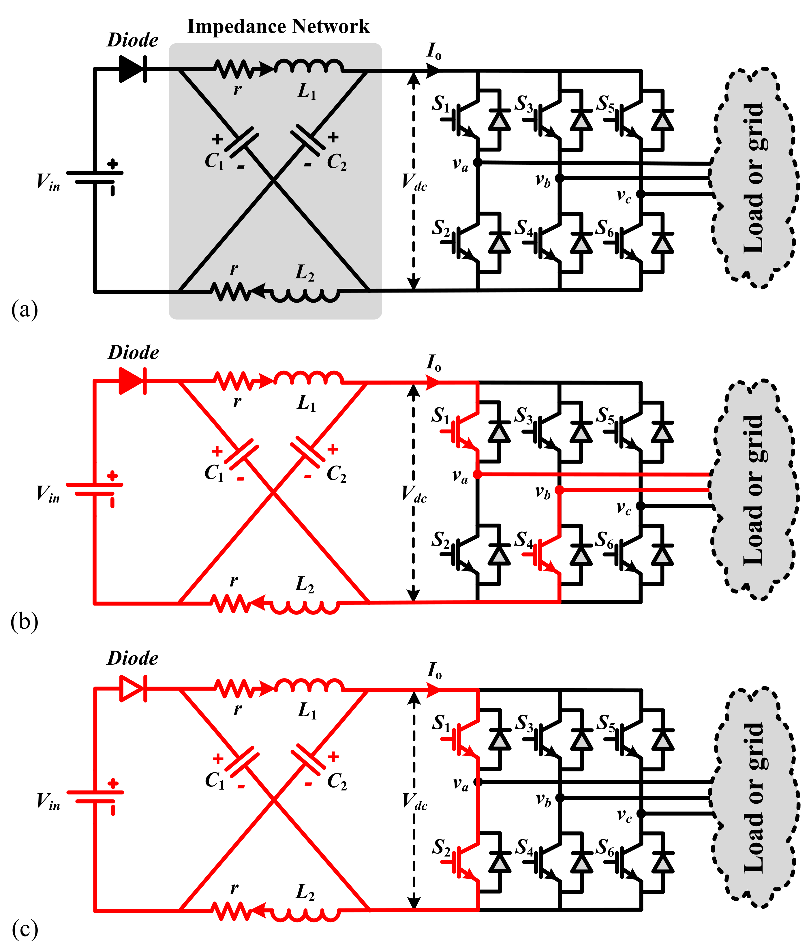
Figure 2. 3-stage simple boost PWM waveform.

Effigy ii. Three-phase simple heave PWM waveform.

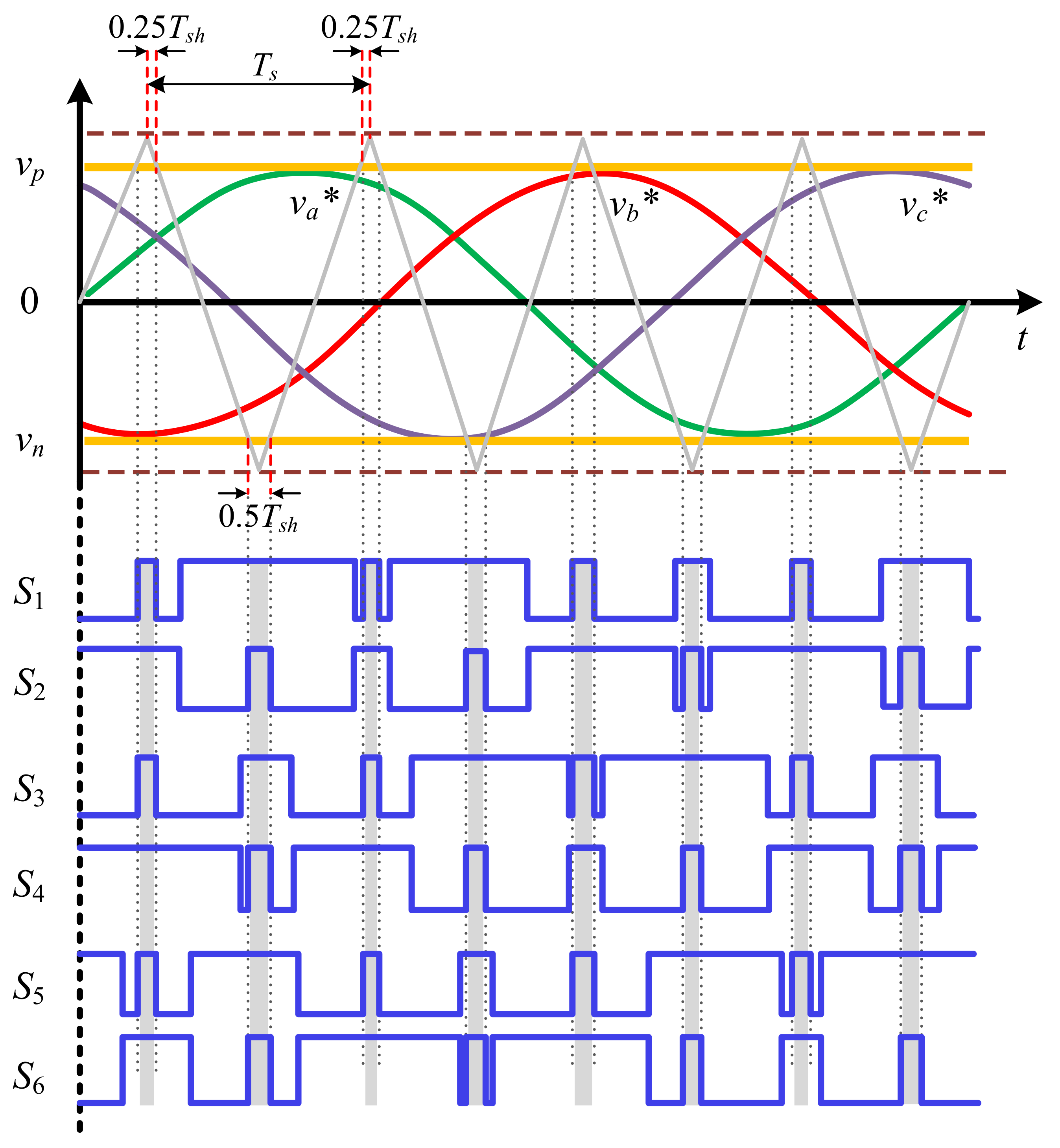
Figure iii. Double-loop control of a ZSI using (a) PI command, (b) land-feedback, and (c) proposed MFAC.

Figure 3. Double-loop command of a ZSI using (a) PI control, (b) state-feedback, and (c) proposed MFAC.

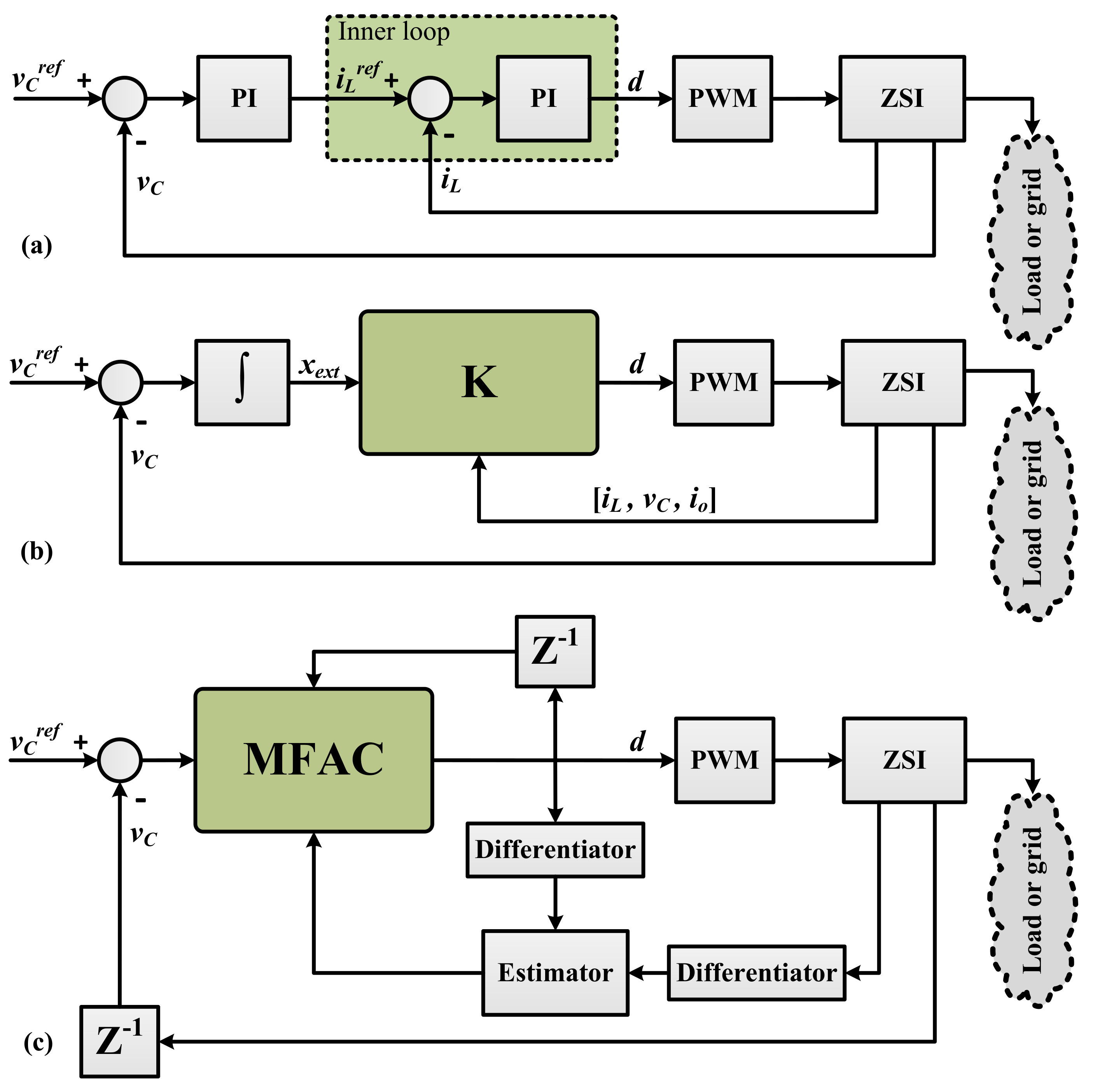
Figure 4. Nominal airtight-loop response for a 4 A load disturbance (

$D=0.4347$

,

$R_o=27$

).

Figure 4. Nominal closed-loop response for a 4 A load disturbance (

$D=0.4347$

,

$R_o=27$

).

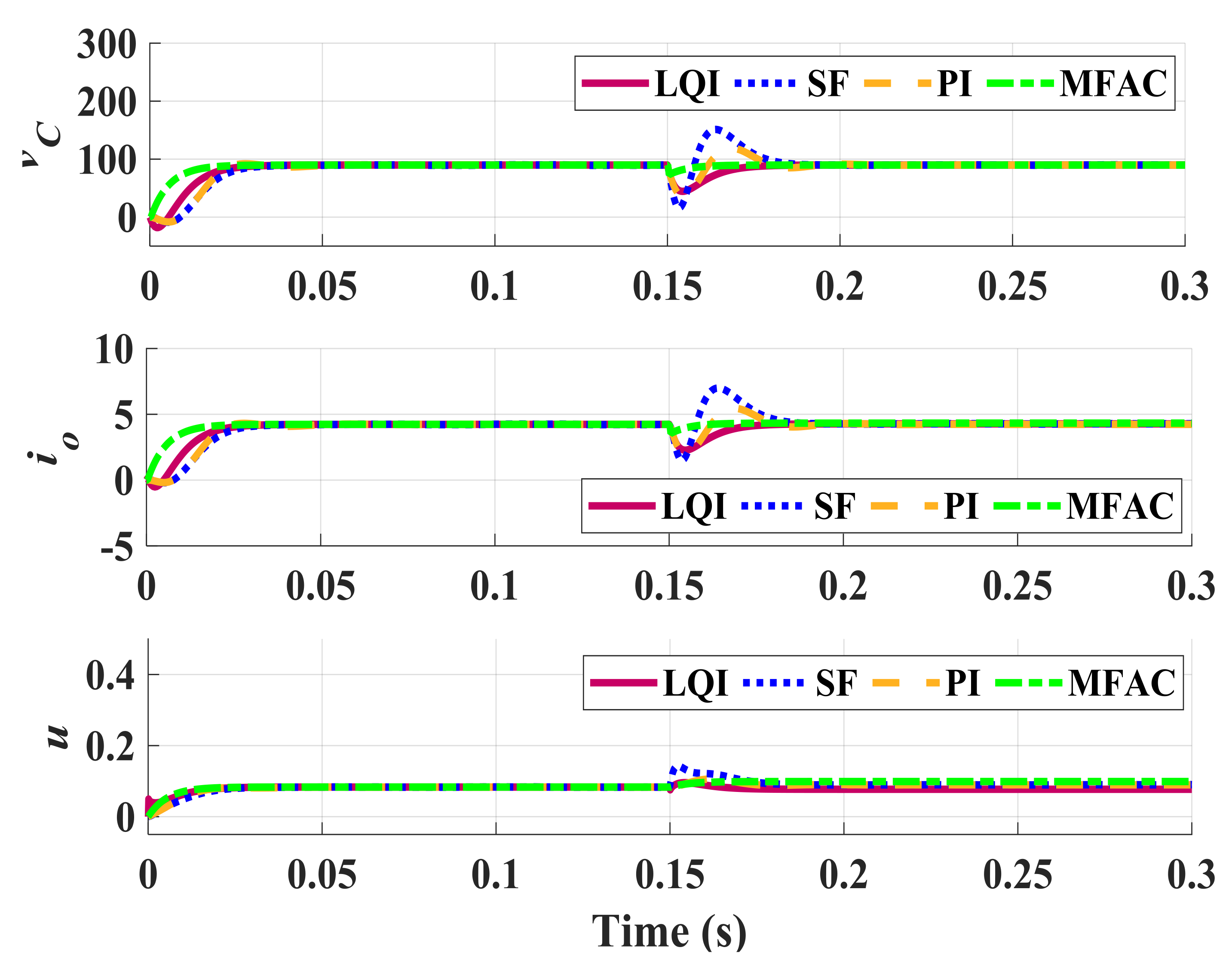
Figure 5. Perturbed airtight-loop response for a four A load disturbance (

$D=0.45$

,

$R_o=\mathrm{lx}$

).

Effigy 5. Perturbed airtight-loop response for a 4 A load disturbance (

$D=0.45$

,

$R_o=\mathrm{lx}$

).

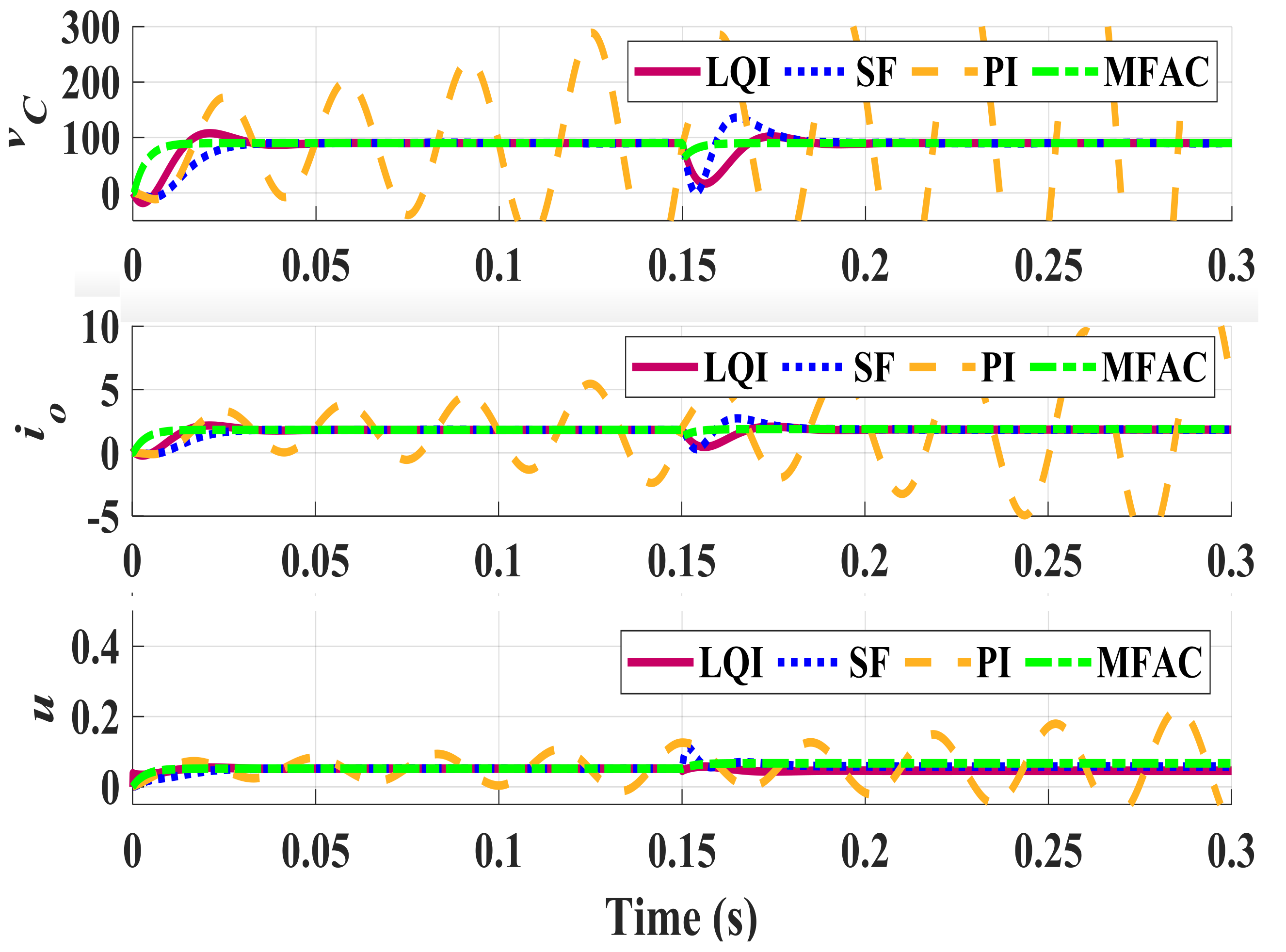
Figure 6. Perturbed closed-loop response for a 4 A load disturbance (

$D=0.4$

,

$R_o=60$

).

Figure 6. Perturbed closed-loop response for a iv A load disturbance (

$D=0.4$

,

$R_o=60$

).

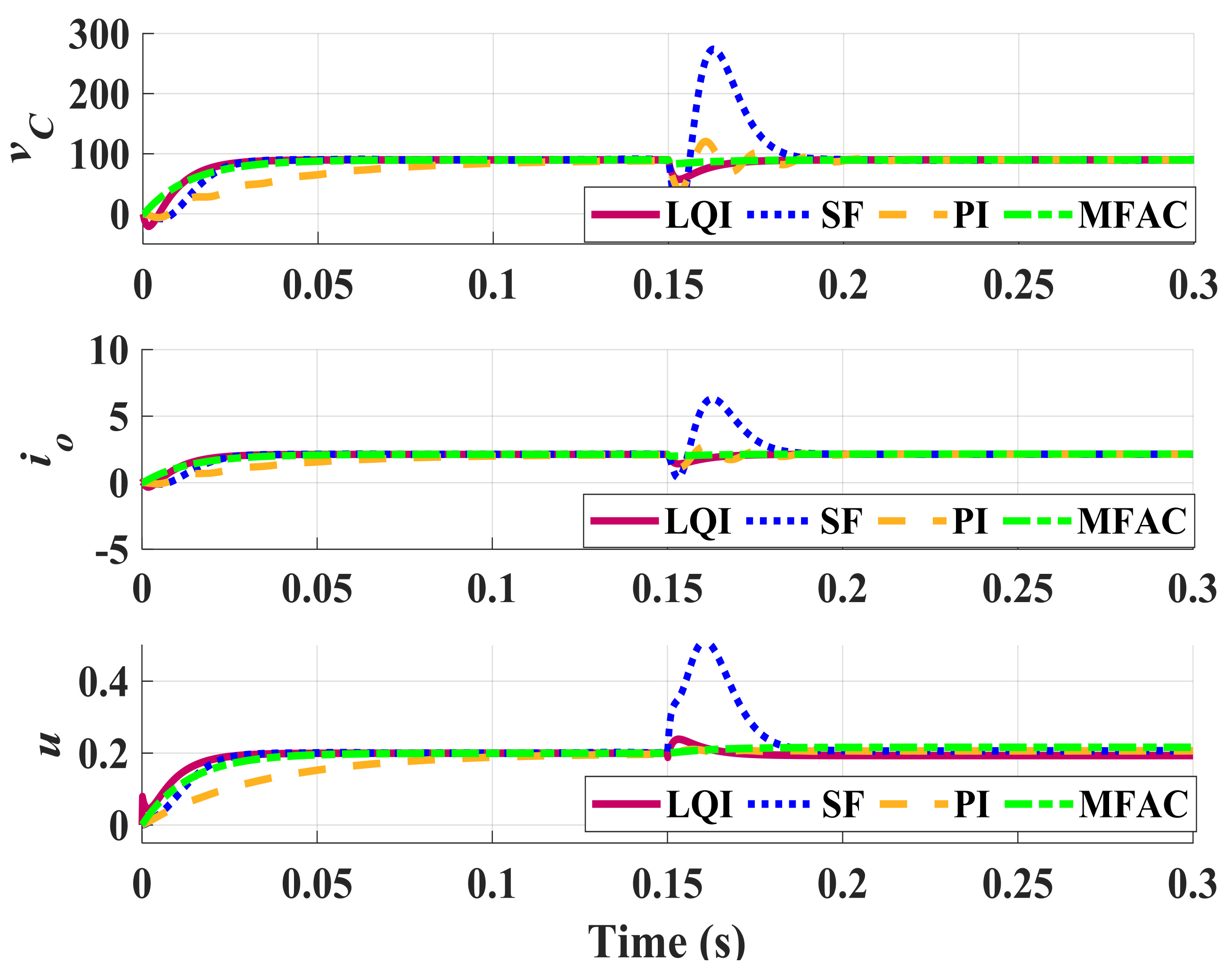
Table 1. Parameters of the inverter in the nominal condition.

Table ane. Parameters of the inverter in the nominal condition.

Parameter	Symbol	Value
Input voltage (5)	$5_{in}$	xx
Shoot-through duty bike	D	$0.4374$
Capacitor voltage (V)	$V_C$	$89.8146$
Inductor electric current (A)	$I_L$	$19.05$
Output current (A)	$I_o$	$4.2362$
Capacitor ($\mathsf{\mu }$F)	C	$92.25$
Inductor (mH)	Fifty	$2.1$
Coupling inductor (mH)	${\mathrm{Fifty}}_o$	$6.6$
Load ($\Omega$)	$R_o$	27
Parasitic resistance ($\Omega$)	r	$0.05$
Switching frequency (KHz)	f	10

Tabular array 2. Metrics of the nominal organization (

$D=0.4374$

and

$R_o=27$

).

Table ii. Metrics of the nominal system (

$D=0.4374$

and

$R_o=27$

).

		Servo Response		Regulatory Response
Controller	Tv set	IAE	MP(%)	IAE	Peak
LQI	0.095	1.325	0	0.637	0
SF	0.083	1.562	0	26.456	62.027
PI	0.128	1.505	ane.984	27.054	29.195
MFAC	0.016	0.869	0	0.112	0

Table 3. Metrics of the perturbed system (

$D=0.45$

and

$R_o=60$

).

Table 3. Metrics of the perturbed organisation (

$D=0.45$

and

$R_o=\mathrm{sixty}$

).

		Servo Response		Regulatory Response
Controller	TV	IAE	MP(%)	IAE	Peak
LQI	0.066	1.656	0	1.197	0
SF	0.092	2.055	0	25.720	48.990
PI	0.968	ten.256	72.331	viii.651	106.560
MFAC	0.116	one.481	0	0.991	0

Table 4. Metrics of the perturbed system (

$D=\mathrm{0.iv}$

and

$R_o=60$

).

Tabular array 4. Metrics of the perturbed system (

$D=0.4$

and

$R_o=60$

).

		Servo Response		Regulatory Response
Controller	TV	IAE	MP(%)	IAE	Peak
LQI	0.142	0.982	0	0.432	0
SF	0.120	1.409	0	2.999	195.893
PI	0.161	two.144	0	0.724	36.837
MFAC	0.116	0.123	0	0.157	0

Publisher'south Note: MDPI stays neutral with regard to jurisdictional claims in published maps and institutional affiliations.

© 2021 by the authors. Licensee MDPI, Basel, Switzerland. This article is an open access article distributed under the terms and conditions of the Creative Commons Attribution (CC BY) license (https://creativecommons.org/licenses/by/4.0/).

We utilise cookies on our website to ensure you become the best experience.
Read more than nigh our cookies hither.

We have just recently launched a new version of our website.
Help us to further meliorate by taking part in this short v minute survey here. hither.

hayesthiskence.blogspot.com

Source: https://www.mdpi.com/1424-8220/21/22/7438/html